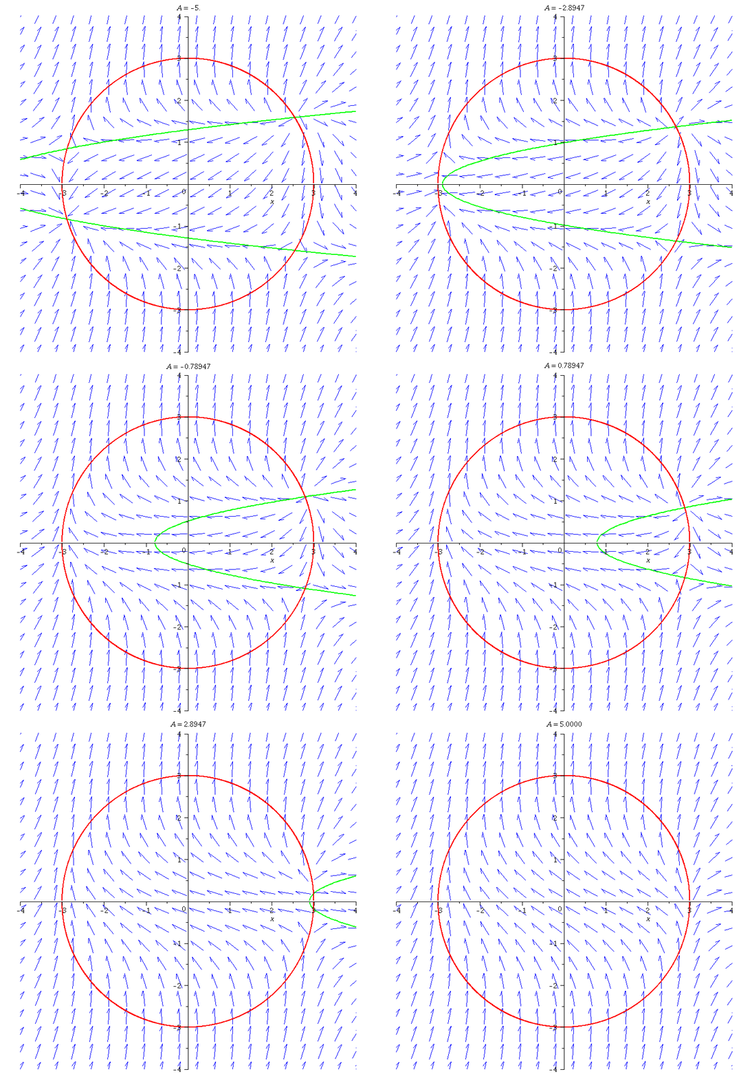
Animation of the bifurcations for system x' = x^2 + y^2 -9, y' = 3y^2 +A-x, as A goes from -5 to 5
| > | with(DEtools):with(plots): |
The red circle marks points where x' = 0. It is fixed.
| > | circle:=plot([sqrt(9-x^2),-sqrt(9-x^2)],x=-4..4,color=red,numpoints=5000,thickness=2): |
Animation a2 has a moving green parabola where y' = 0 with the red circle as background. The parameter A goes from -5 to 5. So, we do not see the first bifurcation.
| > | a2:=animate(plot, [[sqrt((x-A)/3), -sqrt((x-A)/3)],x=-4..4,color=green,thickness=2], A=-5..5,background=circle,view=[-4..4,-4..4],frames=20); |
| (1) |
Animation a1 is the direction field for A -5 to 5.
| > | a1:=animate(dfieldplot, [[D(x)(t)=x(t)^2+y(t)^2-9,D(y)(t)=3*y(t)^2+A-x(t)],[x(t),y(t)],t=0..1,x=-4..4,y=-4..4,color=blue],A=-5..5,frames=20); |
| (2) |
Finally we display the two animations together. Watch closely.
| > | display(a1,a2); |
 |
| > |