Heat Equation on a square plate

Assume the boundary of 1x1 metal square plate are help to 0 degree. We aasume alpha=1.

Let the initial temp be f(x,y) = (x-0.5)^2 + (y-0.5)^2. Below is its graph.

>	with(plots):

>	plot3d( (x-0.5)^2 + (y-0.5)^2, x=0..1, y=0..1);

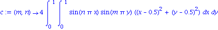
The command below defines the Fourier coeficients.

>	c := (m,n) -> 4*int(int( sin(n*Pi*x) * sin(m*Pi*y) * ((x-.5)^2 + (y-.5)^2),x=0..1),y=0..1);

We plot u(x,y,t) for several values of t and then do an animation.

>	plot3d(sum(sum(c(m,n)*sin(n*Pi*x)*sin(m*Pi*y),m=1..100),n=1..100),x=0..1,y=0..1,title="t=0.0");

>	plot3d(sum(sum(c(m,n)*sin(n*Pi*x)*sin(m*Pi*y)*exp(-(m^2+n^2)*0.01),m=1..100),n=1..100),x=0..1,y=0..1,view=-0.1..0.5,title="t=0.01");

>	plot3d(sum(sum(c(m,n)*sin(n*Pi*x)*sin(m*Pi*y)*exp(-(m^2+n^2)*0.05),m=1..100),n=1..100),x=0..1,y=0..1,view=-0.1..0.5,title="t=0.05");

>	plot3d(sum(sum(c(m,n)*sin(n*Pi*x)*sin(m*Pi*y)*exp(-(m^2+n^2)*0.1),m=1..100),n=1..100),x=0..1,y=0..1,view=-0.1..0.5,title="t=0.1");

For the animation summing out to 100 for m and n was too time consumming, so I just did them out to 10. Thus, the t=0 graph looks rather choppy.

>	animate(plot3d ,[sum(sum(c(m,n)*sin(n*Pi*x)*sin(m*Pi*y)*exp(-(m^2+n^2)*t),m=1..10),n=1..10),x=0..1,y=0..1],t=0..0.3,frames=100);