This is an example done in class. It is #25 in section 3.1: 2y'' + 3y'- 2y = 0, y(0)=1, y'(0)=-b.

> dsolve({2*diff(y(x),x$2)+3*diff(y(x),x)-2*y(x)=0,y(0)=1, D(y)(0)=-b},y(x));

> with(plots):

Click on the plot below. It is an animation. Click on the play arrow to run it. (In this HTML export it seems to run on its own.)

> animate((4/5-2/5*b)*exp(1/2*x)+(1/5+2/5*b)*exp(-2*x),x=-5..5,b=-5..5,frames=50,view=-10..10,thickness=2,color=green);

We can see that for some values of b there is a minimum while for others there is not. We will find all values of b for which there is a minimum. First we will find the minimum value and location for b=1, as warm up.

> plot((2*exp(x/2)+3*exp(-2*x))/5,x=0..2);

> solve(diff((2*exp(x/2)+3*exp(-2*x))/5,x)=0);

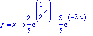
> f := x -> (2*exp(x/2)+3*exp(-2*x))/5;

> f(2/5*ln(6));

> evalf(2/5*ln(6)); evalf(1/2*6^(1/5));

Thus the coordinates of the minimum are approximately (.7167037876, .7154845405).

Now for the general case.

> solve(diff((4/5-2/5*b)*exp(1/2*x)+(1/5+2/5*b)*exp(-2*x),x)=0,x);

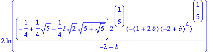
Hmmm? The command returned several roots. Only the first is a real number. But is it required that (1+2b)/(b-2) >0.

This only holds for b in (-1/2, 2).