Direction fields and Solution curves

>	with(DEtools):with(plots):

Warning, the name changecoords has been redefined

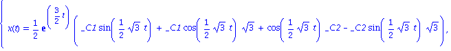
Here is a direction field plot for a linear system: x'(t) = 2x-y,  y'(t) = x+y.

>	dfieldplot([D(x)(t)=2*x(t)-y(t),            D(y)(t)=x(t)+y(t)],            [x(t),y(t)],t=-1..1, x=-10..10,y=-10..10,color=black,thickness=2);

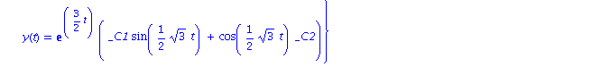
I redo it useing "phaseportrait" instead of "dfieldplot". This allows me to include some solution curves. Two solution curves are shown.

One for initial condition x(0)=y(0)=5 and one for x(0)=-5, y(0)=5. Both curves are plotted as the parameter t goes from -2 to 1.

>	phaseportrait([D(x)(t)=2*x(t)-y(t),               D(y)(t)=x(t)+y(t)],               [x(t),y(t)],t=-2..1,[[x(0)=5,y(0)=5],[x(0)=-5,y(0)=5]], x=-10..10,y=-10..10,color=black,linecolor=[red,blue],thickness=4);

Now we use dsolve to find the general solution explicitly. Then we use a different initial condition and plot the result.

>	system1 := diff(x(t),t) = 2*x(t)-y(t),           diff(y(t),t) =   x(t)+y(t);

>	dsolve({system1});

>	initcond :=x(0)=2,y(0)=3;

>	dsolve({system1,initcond});

>

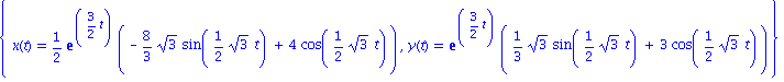
We do a parametric plot. The form of the command is plot[x(t),y(t),t=a..b], options).

>	plot([1/2*exp(3/2*t)*(-8/3*sqrt(3)*sin(1/2*sqrt(3)*t)+4*cos(1/2*sqrt(3)*t)),     exp(3/2*t)*(1/3*sqrt(3)*sin(1/2*sqrt(3)*t)+3*cos(1/2*sqrt(3)*t)),t=-2..1],thickness=3);

>